Reinforcement Learning with Neural Network

1. Introduction

In this tutorial, we’ll explore the basics of reinforcement learning and how we can use neural networks within it. In addition, we’ll develop a small application to go through fundamental concepts.

2. Some Basics

Before we begin, let’s try to understand what we mean by reinforcement learning and neural networks.

2.1. Machine Learning and Reinforcement Learning

Machine learning refers to a class of algorithms that promises to improve automatically based on experience. More generally, machine learning is a part of artificial intelligence, which is the study of intelligent agents founded in 1956.

We can broadly divide machine learning into three categories depending upon the feedback available for the algorithm to learn over time:

• Supervised Learning: The objective of supervised learning is to learn a function that can map the input to output, exploiting from a labeled set of training data.
• Unsupervised Learning: In contrast, unsupervised learning is about learning undetected patterns in the data, through exploration without any pre-existing labels.
• Reinforcement Learning: Finally, the goal of reinforcement learning is to maximize the cumulative reward by taking actions in an environment, balancing between exploration and exploitation.

2.2. Neural Networks and Deep Learning

Now let’s understand what we mean by neural networks. We often employ neural networks as a technique to solve machine learning problems, like supervised learning.

Neural networks consist of many simple processing nodes that are interconnected and loosely based on how a human brain works. We typically arrange these nodes in layers and assign weights to the connections between them. The objective is to learn these weights through several iterations of feed-forward and backward propagation of training data through the network.

So what is deep learning, and how does it relate to neural networks? As we now know, a neural network comprises processing nodes arranged in layers. From just a few nodes and layers, a network can grow into millions of nodes arranged into thousands of layers.

We typically construct these networks to solve sophisticated problems and categorize them as deep learning. When we apply deep learning in the context of reinforcement learning, we often term that as deep reinforcement learning.

3. Reinforcement Learning Primer

Reinforcement learning is about an autonomous agent taking suitable actions to maximize rewards in a particular environment. Over time, the agent learns from its experiences and tries to adopt the best possible behavior.

In the case of reinforcement learning, we limit human interaction to changing the environment states, and the system of rewards and penalties. This setup is known as the Markov Decision Process.

3.1. An Example

To understand this better, let’s take the example of training a pet. We can consider the pet as an autonomous agent. If we’re trying to train the pet in our living room, that can be considered as the environment:

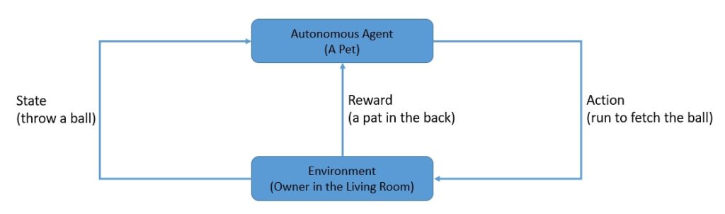
We can throw a ball and expect the pet to run and fetch it. Here, throwing the ball represents a state that the environment presents, and running to fetch it represents an action that the pet may take. Finally, we may reward the pet in the form of a pat on the back or penalize the pet by ignoring it.

We can issue rewards immediately or delay them to some point in the future. Of course, a future reward is often less valuable in the present and hence discounted.

3.2. Types of Environment

Reinforcement learning primarily consists of two types of environments:

• Deterministic: This refers to the case where both the state transition model and reward model are deterministic functions. Simply put, an agent can expect the same reward and next state if it repeats an action in a particular state.
• Stochastic: Stochastic refers to something that has a random probability of occurrence. Within such an environment, if an agent takes action in a state repeatedly, they cannot be guaranteed to receive the same reward or the next state.

3.3. Types of Reinforcement Learning

There are generally two types of reinforcement learning:

• Model-Based: In a model-based algorithm, the agent uses experience to construct an internal model of the transitions and immediate outcomes in the environment, and refers to it to choose appropriate action. The agent can externally receive the state transition and reward probability functions.
• Model-Free: In contrast, in a model-free algorithm, the agent uses experience to learn the policy or value function directly without using a model of the environment. Here, the agent only knows about the possible states and actions in an environment and nothing about the state transition and reward probability functions.

3.4. Value Functions and Policy

The reward is immediate feedback that an agent receives from the environment for an action that it takes in a given state. Moreover, the agent receives a series of rewards in discrete time steps in its interactions with the environment.

The objective of reinforcement learning is to maximize this cumulative reward, which we also know as value. The strategy that an agent follows is known as policy, and the policy that maximizes the value is known as an optimal policy.

Formally, the notion of value in reinforcement learning is presented as a value function:

Here, the function takes into account the discounted future rewards starting in a state under a given policy. We also know this as the state-value function of this policy. The equation on the right side is what we call a Bellman equation, which is associated with optimality conditions in dynamic programming.

3.5. Q-value and Q-learning

Q-value is a measure of the long-term return for an agent in a state under a policy, but it also takes into account the action an agent takes in that state. The basic idea is to capture the fact that the same action in different states can bare different rewards:

Here the function creates a map of the state and action pairs to the rewards. We also know this as the action-value function for a policy.

Q-value is a measure we use in Q-learning, which is one of the main approaches we use toward model-free reinforcement learning. Q-learning emphasizes how useful a given action is in gaining some future reward in a state under a policy.

4. Implementing Reinforcement Learning

Now that we’ve covered enough basics, we should be able to attempt to implement reinforcement learning. We’ll be implementing the q-learning algorithm for this tutorial.

4.1. Test Environment

OpenAI is a company that has developed several tools and technologies for standardization and wider adoption of artificial intelligence. The gym is a toolkit from OpenAI that helps us evaluate and compare reinforcement learning algorithms.

Basically, the gym is a collection of test environments with a shared interface written in Python. We can consider these environments as a game, the FrozenLake environment, for instance. FrozenLake is a simple game that controls the movement of the agent in a grid world:

The rules of this game are:

• The grid consists of 16 tiles set up 4×4
• There is a starting tile (S) and a goal tile (G)
• Some tiles are walkable (F) while others can kill the agent (H)
• Movement of the agent is largely uncontrollable
• The agent is rewarded for finding a walkable path from the starting tile to the goal tile

We’ll be using this environment to test the reinforcement learning algorithm we’re going to develop in the subsequent sections.

4.3. Q-learning Process

Before we start implementing the q-learning algorithm, it’s worthwhile to understand what a typical q-learning process looks like:

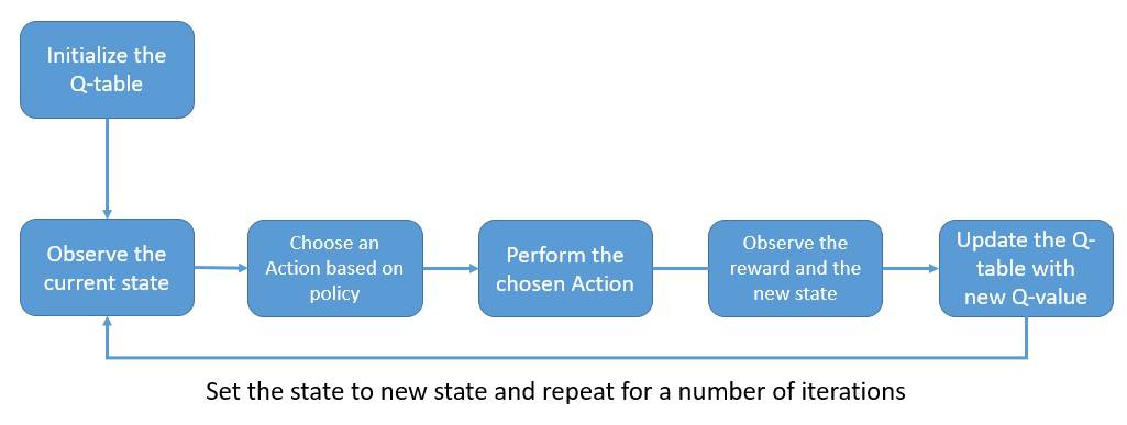
The q-values are stored and updated in a q-table, which has dimensions matching the number of actions and states in the environment. This table is initialized with zeros at the beginning of the process.

As evident from the diagram above, the q-learning process begins with choosing an action by consulting the q-table. On performing the chosen action, we receive a reward from the environment and update the q-table with the new q-value. We repeat this for several iterations to get a reasonable q-table.

4.4. Choosing an Action

We saw earlier that when the process starts, the q-table is all zeros. Hence the action an agent chooses cannot be based on the q-table, it has to be random. However, as the q-table starts to get updated, the agent makes the selection of the action based on the maximum q-value for a state.

This may potentially lock the agent in repeating some of the initial decisions that were not optimal. Essentially, the agent moves from exploration to exploitation of the environment too soon. Therefore, it is necessary to introduce an action selection policy called the .

Here we sample a random number, and if it happens to be less than , the action is chosen randomly. This allows the agent random exploration, which can be very useful, especially in the initial iterations. Of course, we slowly decay the impact of this parameter to lean on the side of exploitation as learning matures.

4.5. Updating the Q-value

We have already seen that the calculation of q-value follows a Bellman equation, but how does it really work? Let’s understand different parts of this equation a little better:

So basically, we keep adding a temporal difference to the current q-value for a state and action pair. There are two important parameters here which are important to choose wisely:

• Learning rate: This is a parameter we can use to control the pace at which our algorithm can learn. We set it between o and 1 with an effective value of 0, meaning no learning at all.
• Discount factor: We saw earlier that a future reward has less importance for actions in the present. We model this using a discount factor, again set between 0 and 1.

4.6. Setting-up the Q-learning Algorithm

Now let’s put all the steps we’ve discussed so far in the form of a program to accomplish the q-learning algorithm. We’ll use Python to develop a basic example for demonstration, primarily because Python has a rich ecosystem of libraries for data manipulation and machine learning.

We’ll begin by making the necessary imports:

import gym
import numpy as np

Next let’s get our test environment, FrozenLake, as discussed earlier:

env = gym.make('FrozenLake-v0')

Now we need to set some learning parameters like the discount factor, ϵ-value and its decay parameter, learning rate, and the number of episodes to run for:

discount_factor = 0.95
eps = 0.5
eps_decay_factor = 0.999
learning_rate = 0.8
num_episodes = 500

The values we chose here are based on experience and must be treated as hyperparameters for tuning. As a last bit of preparation, we need to initialize our q-table:

q_table = np.zeros([env.observation_space.n,env.action_space.n])

4.7. Performing the Q-learning Algorithm

Now we’re ready to start the learning process for our agent in the chosen environment:

for i in range(num_episodes):
    state = env.reset()
    eps *= eps_decay_factor
    done = False
    while not done:
        if np.random.random() < eps or np.sum(q_table[state, :]) == 0:
            action = np.random.randint(0, env.action_space.n)
        else:
            action = np.argmax(q_table[state, :])
        new_state, reward, done, _ = env.step(action)
        q_table[state, action] += 
          reward + 
            learning_rate * 
              (discount_factor * np.max(q_table[new_state, :]) - q_table[state, action])
        state = new_state

Let’s understand what is happening in this block of code:

• We are looping through the chosen number of iterations and reducing the ϵ-value by its decay parameter.
• In each iteration, we’re stepping until the game is done (we may choose to step through a fixed number of times as well).
• We are choosing a random action or an action suggested by the q-table as per action selection policy
• We act and receive the reward and new state from the environment
• Most importantly, we use the Bellman equation to update the q-value for the current state and chosen action in the q-table
• Finally, we set the state as the new state received from the environment and repeat the step

Following the above algorithm a sufficient number of times, we’ll arrive at a q-table that will be able to predict the actions in a game quite efficiently. This is the objective in a q-learning algorithm where a feedback loop at every step is used to enrich the experience and benefit from it.

5. Reinforcement Learning with Neural Networks

While it’s manageable to create and use a q-table for simple environments, it’s quite difficult with some real-life environments. The number of actions and states in a real-life environment can be thousands, making it extremely inefficient to manage q-values in a table.

This is where we can use neural networks to predict q-values for actions in a given state instead of using a table. Instead of initializing and updating a q-table in the q-learning process, we’ll initialize and train a neural network model.

5.1. Selecting a Neural Network Architecture

As we’ve discussed, a neural network consists of several processing nodes fashioned into multiple layers that are typically densely connected.

These layers comprise the following:

• Input Layer: The number of nodes in the input layer is generally fixed and corresponds to the input data, for instance, the number of states in an environment.
• Hidden Layers: There are typically one or more hidden layers in neural network architecture. The number of layers and nodes in each layer are hyperparameters of the architecture.
• Output Layer: Finally, the output layer also has a fixed number of nodes which correspond to the required output, for instance, the number of actions in an environment

Let’s see a simple neural network architecture for the test environment we used earlier in the q-learning algorithm:

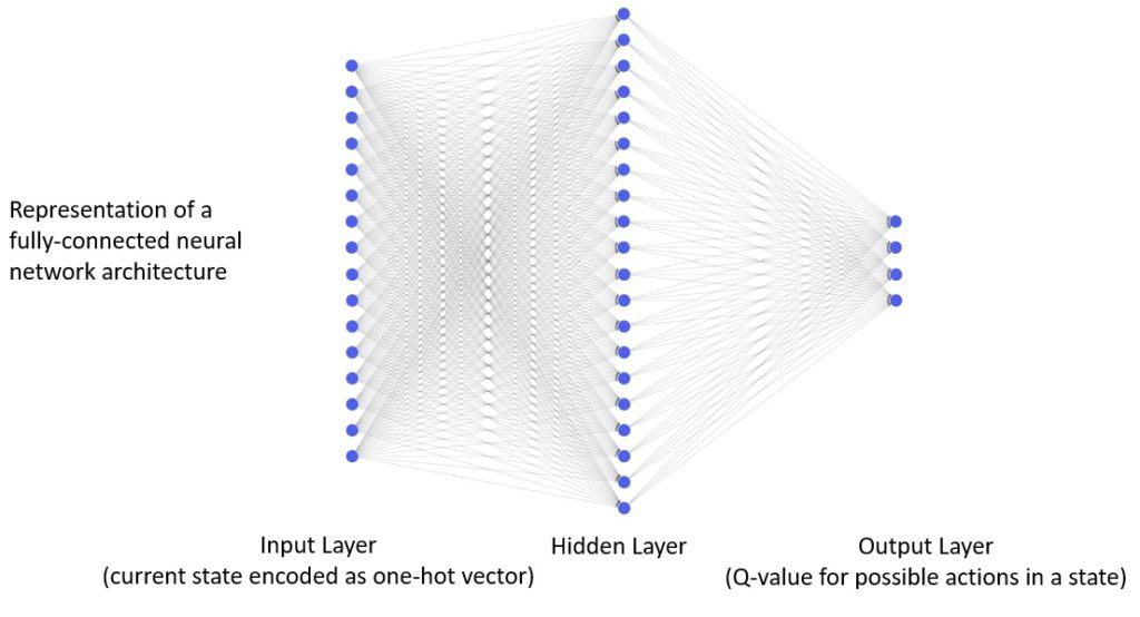
Here our input layer has 16 nodes, which correspond to the number of states in our environment. It receives as input the one-hot encoded state-input vector. There is a single, fully connected hidden layer comprised of 20 nodes. Finally, there is an output layer comprised of 4 nodes corresponding to the number of actions in this environment.

5.2. Choosing the Activation Function

A processing node in the neural network generates the output based on the inputs it receives from the preceding nodes, weights, and biases it learns:

As we can see in the processing node above, it also makes use of an activation function. One of the most important reasons this is necessary is that it provides non-linearity to the output, which is otherwise fairly linear. This non-linearity makes the neural network able to learn complex and real-world patterns.

The choice of activation function in a neural network is a matter of optimization, hence it falls into the list of hyperparameters. However, the nature of input data and the output we desire can help us make a good start. We’ll use the Rectifier Linear Unit (ReLU) as the activation function in the hidden layer and the Linear activation function in the output layer.

5.3. The Loss Function and Optimizer

Neural networks work by iteratively updating the weights and biases of the model to reduce the error in predictions it’s able to make. Therefore, it’s necessary for us to be able to calculate the model error at any point in time. The loss function enables us to do that. Typically, we employ loss functions like cross-entropy and mean-squared-error in neural network models.

The mean-squared-error loss function measures the square value of the difference between the prediction and the target:

The intuition behind calculating the loss function is to take the feedback backward through the network and update the weights. We call this backpropagation, and we can use several algorithms to achieve it, beginning with the classical stochastic gradient descent. Some algorithms are computationally more efficient with lesser memory requirements, like Adam (derived from Adaptive Moment Estimation). We’ll use this in the model for our algorithm.

5.4. Setting up Q-learning with Neural Network

Keras is a higher-level library that works over a data-flow computation library like Tensorflow or Theano. We’ll use Keras to build the q-learning algorithm with the neural network.

The overall structure of the q-learning algorithm will remain the same as we’ve implemented before. The key changes will be in using a neural network model instead of a q-table, and how we update it every step.

Let’s begin by importing the necessary routines:

import gym
import numpy as np
from keras.models import Sequential
from keras.layers import InputLayer
from keras.layers import Dense

Then we’ll get our test environment, FrozenLake, for running the algorithm:

env = gym.make('FrozenLake-v0')

Next, we’ll set up some necessary hyperparameters with sensible defaults:

discount_factor = 0.95
eps = 0.5
eps_decay_factor = 0.999
num_episodes=500

There is nothing new here; however, the next step is to set up the neural network model in Keras. We can also appreciate how simply Keras defines a complex model like this:

model = Sequential()
model.add(InputLayer(batch_input_shape=(1, env.observation_space.n)))
model.add(Dense(20, activation='relu'))
model.add(Dense(env.action_space.n, activation='linear'))
model.compile(loss='mse', optimizer='adam', metrics=['mae'])

This is exactly what we discussed earlier on choosing the neural network architecture for such jobs. The main thing to note is the use of Keras class Sequential, which allows us to stack layers one after another in our model.

5.5. Performing Q-learning with Neural Network

Now that we’ve performed all the necessary set up, we’re ready to implement our q-learning algorithm with the neural network:

for i in range(num_episodes):
    state = env.reset()
    eps *= eps_decay_factor
    done = False
    while not done:
        if np.random.random() < eps:
            action = np.random.randint(0, env.action_space.n)
        else:
            action = np.argmax(
              model.predict(np.identity(env.observation_space.n)[state:state + 1]))
        new_state, reward, done, _ = env.step(action)
        target = reward + 
          discount_factor * 
            np.max(
              model.predict(
                np.identity(env.observation_space.n)[new_state:new_state + 1]))
        target_vector = model.predict(
          np.identity(env.observation_space.n)[state:state + 1])[0]
        target_vector[action] = target
        model.fit(
          np.identity(env.observation_space.n)[state:state + 1], 
          target_vec.reshape(-1, env.action_space.n), 
          epochs=1, verbose=0)
        state = new_state

The algorithm is quite similar to what we implemented earlier; therefore, we’ll only discuss the salient changes neural networks introduce:

• Note that we’re choosing an action based on the as before, but using the neural network model to make a prediction.
• We’re calculating the target value based on the Bellman equation using the model prediction for the new state.
• Finally, we’re using the one-hot encoded current state, and the target value converted as a vector to train the model on a single step.

If we run this algorithm for a sufficient number of iterations, we’ll have a neural network model that can predict the action for a given state in a game with better accuracy. Of course, a neural network model is much more capable of recognizing complex patterns than a simple q-table.

6. Conclusion

In this article, we discussed the basics of reinforcement learning. We explored the q-learning algorithm in particular detail.

Finally, we examined neural networks and how they are beneficial in reinforcement learning.