What Is a Loop Invariant? | Baeldung on Computer Science

1. Introduction

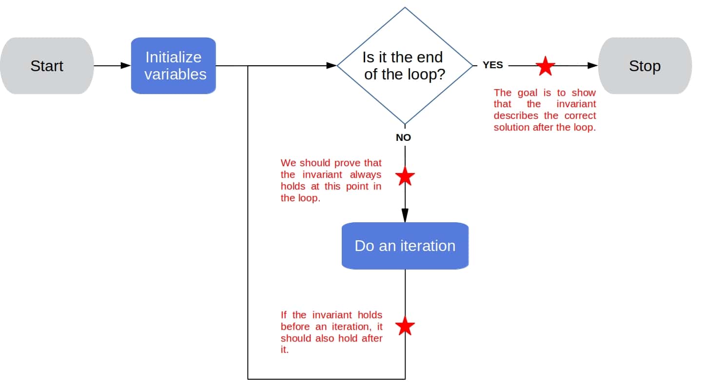
In this tutorial, we’ll explain what’s a loop invariant and how we can use it to prove the correctness of our algorithms.

2. What’s a Loop Invariant For?

A loop invariant is a tool used for proving statements about the properties of our algorithms and programs. Naturally, correctness is the property we’re most interested in. We should be sure that our algorithms always produce correct results before putting them to use.

3. What’s a Loop Invariant and How Do We Prove It?

A loop invariant is a statement about an algorithm’s loop that:

is true before the first iteration of the loop and
if it’s true before an iteration, then it remains true before the next iteration.

If we can prove that those two conditions hold for a statement, then it follows that the statement will be true before each iteration of the loop. Furthermore, it follows that the last iteration won’t affect the invariant, so the two conditions ensure that the invariant is true after the loop as well.

As many algorithms do the actual work in the main loop updating their solution iteratively, the invariant we’re after will state a property of the variable(s) holding the solution. Additionally, the invariant should establish a meaningful relationship between the variable(s) and the number of iterations done. That relation should show that the solution contained in the variable(s) after the loop ends is indeed the correct solution the algorithm was supposed to find.

3.1. How to Formulate a Loop Invariant?

Let’s say that we want to sum an array of real numbers:

algorithm sumArray(a):
    // INPUT
    //    a = an array of n real numbers
    // OUTPUT
    //    The sum of all elements of a

    s <- 0
    for i <- 1 to n:
        s <- s + a[i]
    return s

To be sure that our algorithm works, we should prove that after the loop ends, $s$ is equal to the sum of the numbers in $a$ :

$s = \sum_{i=1}^{n}a_i$

One way to do so is to formulate a loop invariant about variable $s$ :

At the beginning of the $\boldsymbol{i}$ -th iteration, $\boldsymbol{s}$ is equal to the sum of the first $\boldsymbol{i-1}$ elements of $\boldsymbol{a}$ .

How do we check if this is a good invariant? We should verify that the invariant, applied to $s$ after the loop, describes the correct solution. In this example, the loop ends when $i=n+1$ , so the invariant states that at the end of the loop

$s=\sum_{i=1}^{n}a_i$

which is what we want our algorithm to return. So, we identified the invariant we should prove, but, how do we come up with proof?

3.2. How to Prove a Loop Invariant

Proving an invariant is similar to mathematical induction.

The requirement that the invariant hold before the first iteration corresponds to the base case of induction.

The second condition is similar to the inductive step.

But, unlike induction that goes on infinitely, a loop invariant needs to hold only until the loop has ended.

Unfortunately, as each algorithm is unique, there is no universal recipe for writing proofs. All the proofs will have the same structure:

prove that the invariant holds before the first iteration
prove that if the invariant holds before an iteration, then it also holds before the next one

but each step in the process will depend on the actual algorithm:

For Algorithm 1, we’d prove the invariant in two steps.

At the beginning of the loop, $\boldsymbol{i=1}$ and $\boldsymbol{s=0}$ . The sum $\sum_{j=1}^{0}a_j$ is the sum of no numbers. We can use $0$ as its value, so we see that the invariant holds before the first iteration.

Let’s say that the invariant holds at the beginning of the $\boldsymbol{i}$ -th iteration:

$s=\sum_{j=1}^{i-1}a_j$

During the iteration, we add $a_i$ to $s$ , so we get

$s=a_i+\sum_{j=1}^{i-1}a_j\right=\sum_{j=1}^{i}a_j$

at the end of the iteration. The end of iteration $i$ is the same as the beginning of iteration $i+1$ , so the second condition is also fulfilled.

As we’ve shown that

$s=\sum_{i=1}^{n}a_i$

at the end of the loop, proving the invariant also verified that our algorithm was correct.

If the loop is a for–loop, the beginning of an iteration is the point after the loop counter is incremented, but before the loop termination test. That also applies to checking the invariant before the loop.

Let’s now work out two more examples.

4. Sum of Two Binary Numbers

Let’s say that we have two $n$ -bit binary numbers: $\boldsymbol{x} = x_n,x_{n-1},\ldots, x_1$ and $\boldsymbol{y} = y_n,y_{n-1},\ldots, y_1$ ( $x_i,y_i\in\{0,1\}$ for each $i$ ). The result of their addition is an $n+1$ -bit binary number $\boldsymbol{z}=z_{n+1},z_{n},z_{n-1},\ldots, z_1$ . We can calculate each digit $z_i$ by adding $x_i$ and $y_i$ together with the carryover from $z_{i-1}$ :

algorithm sumBinaryNumbers(x, y):
    // INPUT
    //     x, y = two n-bit binary numbers
    // OUTPUT
    //     z = the sum of x and y

    c <- 0
    z <- reserve n bits for the result
    for i <- 1 to n:
        z[i] <- (x[i] + y[i] + c) mod 2
        c <- (x[i] + y[i] + c) div 2
    z[n+1] <- c
    
    return z

4.1. Formulate the Loop Invariant

To verify its correctness, we’ll use a loop invariant which states that $\boldsymbol{z}$ is the correct result:

At the beginning of the $\boldsymbol{i}$ -th iteration, the number $\boldsymbol{c_i,z_{i-1},z_{i-2},\ldots,z_1}$ is the sum of $\boldsymbol{x_{i-1},x_{i-2},\ldots,x_1}$ and $\boldsymbol{y_{i-1},y_{i-2},\ldots,y_1}$ .

Would proving this invariant make sure that the returned variable, $\boldsymbol{z}$ , really is the correct solution? At the end of the loop, $i=n+1$ , so per the invariant, the number $c,z_{n},z_{n-1},\ldots,z_1$ would be the sum of $x_{n},x_{n-1},\ldots,x_1$ and $y_{n},y_{n-1},\ldots y_1$ . This means that we chose the right invariant for if we prove it, then we’ll also prove that our algorithm is correct.

4.2. Prove the Invariant Holds Before the First Iteration

Before the first iteration of the main loop, $i=1$ and $c=0$ . Since there is no digit $z_0$ , we take $c=0$ to be the solution and the only digit. Similarly, there are no digits $x_0$ and $y_0$ in $\boldsymbol{x}$ and $\boldsymbol{y}$ so we practically have no numbers to add. We can treat the sum of no numbers as being equal to $0$ . So, the invariant is true before the first iteration.

4.3. Prove the Invariant Remains True After Each Iteration

If the invariant holds at the beginning of iteration $\boldsymbol{i}$ , does it hold at the beginning of iteration $\boldsymbol{i+1}$ ? Let’s assume that $c,z_{i-1},z_{i-2},\ldots,z_1$ is indeed the sum of $x_{i-1},x_{i-2},\ldots,x_1$ and $y_{i-1},y_{i-2},\ldots, y_1$ . How do we compute digit $z_i$ ? We sum digits $x_i$ and $y_i$ together with the carryover term $c$ from the last iteration in which we computed $z_{i-1}$ . When we divide $x_i +y_i + c$ by $2$ , the integer remainder is digit $z_i$ and the quotient is the carryover term $c$ for the next iteration, which proves that the invariant will be true at the beginning of the next iteration:

$old\ c$	$x_i$	$y_i$	$z_i$	$new\ c$
0	0	0	0	0
0	0	1	1	0
0	1	0	1	0
0	1	1	0	1
1	0	0	1	0
1	0	1	0	1
1	1	0	0	1
1	1	1	1	1

5. Insertion Sort

The Insertion Sort Algorithm is an $O(n^2)$ sorting algorithm:

algorithm insertionSort(a):
    // INPUT
    //     a = an array of n real numbers (1-based indexing)
    // OUTPUT
    //     The non-decreasingly ordered permutation of a

    for j <- 2 to n:
        x <- a[j]
        i <- j - 1
        while i > 0 and a[i] > x:
            a[i + 1] <- a[i]
            i <- i - 1
        a[i + 1] <- x
    return a

5.1. Define the Loop Invariant

Let’s define the main loop’s invariant:

At the start of each iteration of the for–loop, the subarray $\boldsymbol{a[1], a[2], \ldots, a[j-1]}$ consists of the elements originally in $\boldsymbol{a}$ on the positions $\boldsymbol{1}$ through $\boldsymbol{j-1}$ , but in sorted order.

Is this a good invariant? At the end of the for–loop, $j=n+1$ , so the invariant will state that the whole $a$ is sorted.

5.2. Prove the Invariant Holds Before the First Iteration

We see that $j=2$ before the first iteration. So, the invariant claims that [ $a_1$ ] is a sorted array. It (trivially) holds just as we assumed that zero can be taken as the sum of no numbers.

5.3. Prove the Invariant Remains True After Each Iteration

Let’s suppose that $a[1] \leq a[2] \leq \ldots \leq a[j-1]$ and that we set $x$ to $a[j]$ at the beginning of an iteration. We need to prove that after the inner while–loop, the elements $a[i+1], a[i+2], \ldots, a[k-1]$ are greater than $x$ (the original $a[j]$ ) and that $a[1], a[2], \ldots, a[i]$ are lower than or equal to $x$ .

We can formally prove that by proving the corresponding loop invariant for the while–loop. But, informally, we see that the while–loop moves the elements of $a$ one place to the right as long as they’re greater than $x$ . When the loop stops, that’s because it found the element ( $a[i]$ ) which is lower than or equal to $x$ . Therefore, all the elements which were moved to the right, and those are $a[i+1], a[i+2],\ldots,a[j-1]$ , are greater than $x=a[j]$ . All those unaffected by the while–loop are lower than $a[j]$ : $a[1], a[2], \ldots, a[i]$ . So, when we place $a[j]$ at the $i$ -th position in $a$ , the whole subarray will be sorted.

6. Trivial Statements

In proving that an invariant holds before the first iteration, we usually rely on statements such as:

The sum of no numbers is equal to zero.
An array that has only one element is sorted.

Those are the statements we can take to be true without proof. They’re called trivial and are widely used in proving base cases.

7. Conclusion

In this article, we explained what’s a loop invariant and showed how to prove it. We also worked out a couple of examples to illustrate how we can use a loop invariant to verify an algorithm’s correctness.

Learn Java Collections

Learn Spring

Learn Maven

View All Courses

Core Concepts

Operating Systems

Neural Networks

Graph Theory

Latex

Full Archive

About Baeldung