Topic Modeling with Latent Dirichlet Allocation

1. Overview

In this tutorial, we’ll learn about topic modeling, some of its applications, and we’ll dive deep into a specific technique named Latent Dirichlet Allocation.

A basic understanding of multivariate probability distributions would be helpful background knowledge.

2. Topic Modeling

2.1. What Is Topic Modeling?

Simply put, the topic of a text is the subject, or what the text is about.

Topic modeling is an unsupervised machine learning method receiving a corpus of documents and producing topics as mathematical objects.

Once the topic model is created, we can express documents as a combination of the discovered topics. Let’s see an example:

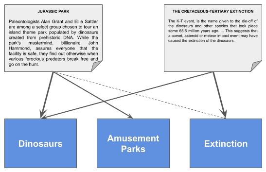
In this example, each document is connected to every topic with different weights. Therefore, we could represent a document as a vector, whose columns are the degree of connection to every topic.

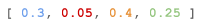
Imagine we want to model “Jurassic Park” as a combination of topics in this proportion:

“Dinosaurs”: 97%
“Amusement Parks”: 49%
“Extinction”: 10%

In that case, the vector representing this document would be [0.97, 0.49, 0.1]

What we just learned is that topic modeling can be used to obtain an embedding vector from a document.

2.2. Applications

Topic modeling has a number of different interesting applications:

Field understanding
Find changes or new trends in our field
Encode text as vector embeddings
Search Personalization
Modeling users’ preference for search
Compare documents
Finding the author of a specific text
Prediction and Interpretation of social activity
Sentiment Analysis
Machine Translation

2.3. Specific Techniques

These are the most widely used techniques for topic modeling:

NMF (Non-Negative Matrix Factorization)
LSA (Latent Semantic Analysis)
PLSA (Probabilistic Latent Semantic Analysis)
LDA (Latent Dirichlet Allocation)
lda2vec
tBERT (Topic BERT)

3. Latent Dirichlet Allocation

3.1. Introduction

Latent Dirichlet Allocation (LDA) is a statistical generative model using Dirichlet distributions.

We start with a corpus of $M$ documents and choose how many $K$ topics we want to discover out of this corpus.

The output will be the topic model, and the $M$ documents expressed as a combination of the $K$ topics.

In a nutshell, all the algorithm does is finding the weight of connections between documents and topics and between topics and words.

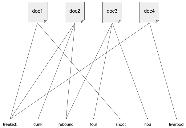
Let’s see it in a visual representation. Imagine this is our word distribution over documents:

For $K = 2$ , an LDA model could look like this:

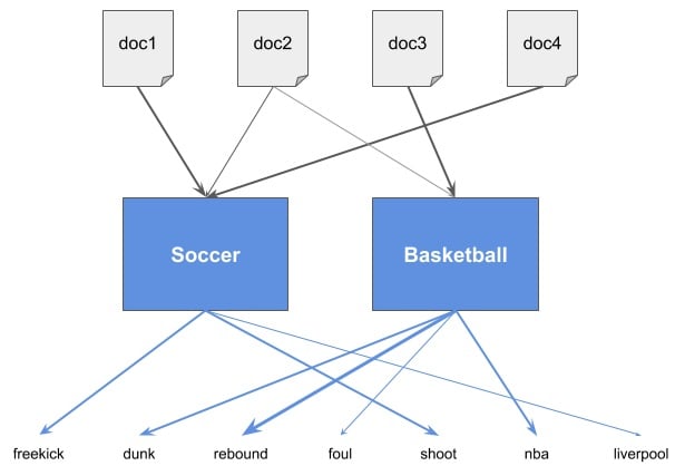
We see how the algorithm created an intermediate layer with topics and figured out the weights between documents and topics and between topics and words. Documents are no longer connected to words but to topics.

In this example, each topic was named for clarity, but in real life, we wouldn’t know exactly what they represent. We’d have topics 1, 2, … up to $K$ , that’s all.

If we want to get an intuition about what each of the topics is about, we’ll need to carry on a more detailed analysis. But fear not, we’ll learn how to do that a bit later!

3.2. Why Dirichlet Distributions?

Dirichlet Distributions encode the intuition that documents are related to a few topics.

In practical terms, this results in better disambiguation of words and a more precise assignment of documents to topics.

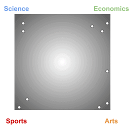
Let’s suppose we have the topics:

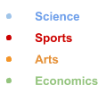
In a random distribution, documents would be evenly distributed across the four topics:

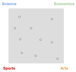
This means documents have the same probability of being about one specific topic than to all topics at the same time.

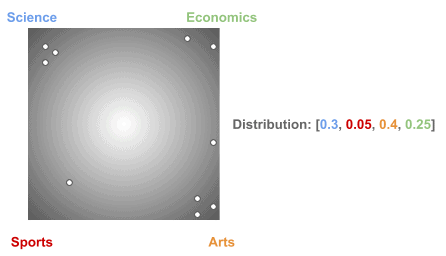
In real life, however, we know they are more sparsely distributed, like this:

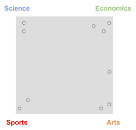
You can see most documents are tied to just one topic, while there’s still some probability to belong to multiple ones, like the document halfway between Economics and Arts.

And so happens between topics and words:

Dirichlet distributions model this behavior in a very natural way.

3.3. What Are Dirichlet Distributions

A Dirichlet distribution $\pmb{Dir(\alpha)}$ is a way to model a Probability Mass Function, which gives probabilities for discrete random variables.

Confused? Let’s see the example of rolling a die:

It is a discrete random variable: The result is unpredictable, and the values can be 1, 2, 3, 4, 5, or 6.
For a fair die, a PMF would give these probabilities: [0.16, 0.16, 0.16, 0.16, 0.16, 0.16]
For a biased die, a PMF could return these probabilities: [0.25, 0.15, 0.15, 0.15, 0.15, 0.15], where obtaining a one is higher than the other sides.

In the example with documents, topics, and words, we’ll have two PMFs:

${\theta_{d}}$ : the probability of topic k occurring in document d
${\varphi_{k}}$ : the probability of word w occurring in topic k

The $\pmb{\alpha}$ in $Dir({\alpha})$ is named concentration parameter, and rules the trend of the distribution to be uniform $({\alpha} = 1)$ , concentrated $({\alpha} > 1)$ , or sparse $({\alpha} < 1)$ .

This would be a distribution with ${\alpha} = 1$ :

Using a concentration parameter ${\alpha} > 1$ , it would look like this:

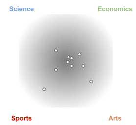
Using ${\alpha} < 1$ , however, we’ll obtain something like this:

which is exactly what we want.

So, by using a concentration parameter ${\alpha} < 1$ , these probabilities will be closer to the real world. In other words, they follow Dirichlet distributions:

${\theta_{d}} \approx Dir(\alpha)$
${\varphi_{k}}\approx Dir(\beta)$

where ${\alpha}$ and ${\beta}$ rule each distribution and both have values $< 1$ .

3.4. A Dirichlet Distribution Is Actually a Family of Distributions

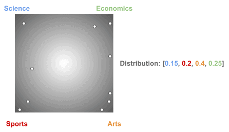
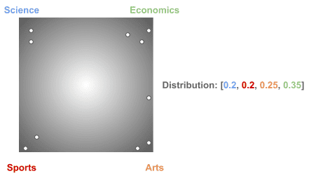
Now, a very important point: using the same concentration parameter $\pmb{\alpha}$ , we obtain many different distributions of documents over topics.

So, why using a fixed concentration parameter? Because it guarantees that documents will be linked to a few topics and topics to a few words.

Next, let’s see some different distributions we could obtain using the same ${\alpha} < 1$ :

Actually, the choice of these specific multinomial distributions is what makes an LDA model better or worse.

They get adjusted during the training process to make the model better.

3.5. Generating New Documents

LDA is a generative model, so it’s able to produce new documents. But bear in mind it’s a statistical model, so the generated document most times won’t make sense from a linguistic point of view.

To better understand how this works, let’s illustrate with an example.

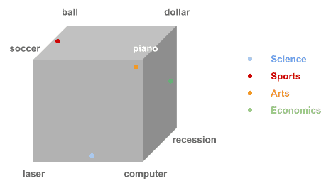
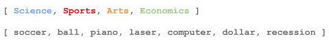
Suppose we have these topics and words:

We start with the distribution D1 of documents over topics:

And the distribution D2 of topics over words:

First, we’re going to sample a few topics from distribution D1, according to its probabilities:

Now, let’s do the same with words from distribution D2:

Finally, all we have to do is going over each sample topic and choose a random word from the sample words for that topic:

1. Randomly pick the first topic from the sample list, i.e., “Science”. Now, pick a random word from the Science sample words. Let’s say “laser”.

2. Next, pick the second random sample topic, i.e., “Economics“, and get a random word from the Economics sample list. Let’s say “recession”.

3. We proceed this way until we reach the last sample topic, obtaining a list of words:

Our sample document would be then:

D = "laser recession piano dollar piano piano laser computer soccer piano"

which doesn’t make sense as human-readable text, but it respects our model’s probabilities.

3.6. Making Sense out of Topics

Once the $K$ topics are found, how can we know what they represent?

LDA will produce a distribution of topics over words. By analyzing that distribution, we can extract the most frequent words for a topic and get an idea of what it is about.

In the previous example with $K = 4$ and words:

$V = \{soccer, ball, piano, laser, computer, dollar, recession\}$

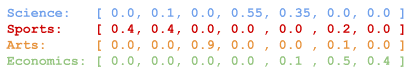
we obtained the distribution:

Topic 1:   [0.0, 0.1, 0.0, 0.55, 0.35, 0.0, 0.0]
Topic 2:   [0.4, 0.4, 0.0, 0.0 , 0.0 , 0.2, 0.0]
Topic 3:   [0.0, 0.0, 0.9, 0.0 , 0.0 , 0.1, 0.0]
Topic 4:   [0.0, 0.0, 0.0, 0.0 , 0.1 , 0.5, 0.4]

Let’s go one topic at a time:

Topic 1: The most frequent words are laser and computer, so it could be about technology or science
Topic 2: The most frequent words are soccer and ball, so it seems to be clearly linked to sports
Topic 3: The most frequent word is piano, so the topic could be probably music
Topic 4: The most frequent words are dollar and recession, so the topic will be related to economics

3.7. Training a Model with Gibbs Sampling

Finally, let’s just outline the intuition behind the training process with Gibbs Sampling:

Randomly assign a topic to each word in the initial documents
Reassign each word topic so that each document contain the least possible topics
Reassign each word topic so that each word is assigned the least possible topics

For those interested in learning all about it, please have a look here.

4. Conclusion

In this tutorial, we learned about topic modeling, some of its applications, and the most widely used techniques to do it.

We also learned about LDA, what are Dirichlet distributions, how to generate new documents and find what each topic represents.

Learn Java Collections

Learn Spring

Learn Maven

View All Courses

Core Concepts

Operating Systems

Neural Networks

Graph Theory

Latex

Full Archive

About Baeldung